Increased Productivity Example #1
A.C. Motor Design
__________
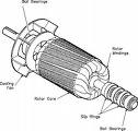
Figure 1 is a case study of re-engineering -- an A.C. motor design simulation that was reapplied as an optimization program and fully tested in about an hour. The original program had been used for trial and error design calculations by a west coast manufacturer. Restructuring this mature engineering model into a design optimization program, only required introducing a FIND statement that defined a constrained optimization problem with 12 unknown parameters and 7 constraints. A FIND statement invokes a solution technique or solver that consists of automatic differentiation with a numerical algorithm. The solver involved in this case is a nonlinear programming algorithm called THOR. Figure 2 (part of output) is a report automatically generated by the solver, THOR, summarizing the iteration steps. This partial summary shows initial guesses of the parameters and the final results.
This case study illustrates the economic benefits of AD based software for reapplying existing application software in a higher-productivity mode. The existing engineering simulation model was used "as is". It was automatically elevated to optimization by the hidden differential arithmetic. There was no mathematical analysis or algorithm design required. Because this was a re-engineering of an existing program, no debugging was necessary, and since the optimization solvers are interchangeable, different algorithms could be substituted to verify solution correctness.
Increased Productivity Example #1 Source Code:
Figure 1. Calculus Code ... A.C. Motor (Optimal) Design
global all
problem acmotor
  dimension cns(7)
  dynamic botm, bnd
  call input
  call design
  print *, '---------------initial design---------------'
  call output
  Find coiltrns, ! number of turns per coil
&     EPDIAM,     ! Separating diameter
&     STASLOTW,   ! Stator slot opening width
&     ROTSLOTW,   ! Rotor slot opening width
&     AIRGAP,     ! Air gap
&     STATOOTW,   ! Stator tooth width
&     STABAKIR,   ! Stator back iron
&     ROTTOOTW,   ! Rotor tooth width
&     ROTBAKIR,   ! Rotor back iron
&     STASLOTO,   ! Stator slot opening depth
&     ROTSLOTO,   ! Rotor slot opening depth
&     SLIP        ! Slip
&   in DESIGN; by thor(TCON);
&   with bounds BND; and lowers BOTM;
&   holding CNS; to maximize EFF
  print *, '----------------optimized design-----------------'
  call output
end

model design
  f1 = 231258.0438 / coiltrns
  q1 = sepdiam * pi / 56 : q2=sepdiam * pi / 69 : q3=sepdiam * pi / 28
  c1 =q1/((q1-staslotw)+(staslotw *(.7 -(.036 * staslotw/ airgap))))
  c2 =q2/((q2-rotslotw)+(rotslotw *(.7-(.036 * rotslotw/airgap))))
  crnol = f1 * airgap * c1 * c2 / (6.96 * coiltrns * q3)
  q4 = (statorod - stabakir - stabakir - sepdiam - .1) / 2 - .01
  q5= (sepdiam+q4+.1) * pi / 56 - statootw - .016 : a3=q4 * q5
  z1 = 7000 * a3
  q6 = coiltrns * 2 / z1 : z3= - 2 : z4=32+z3 : q7=1.26**z3 * 162
  q8=64 / 1.26**z3 : z5=stacklen+stacklen+pi * statorod / 14
  rdc =z5 * coiltrns * 28 * q7 / 12000
  v1 = (sepdiam - .06 - rotorid - rotbakir - rotbakir) / 2
  v2 = (sepdiam - .06 - v1) * pi / 69 - rottootw
  a4 = v1 * v2 : r2 = (.0133 / a4) * (stacklen / 12000) * u1
  rrot= (56 * coiltrns)**2 * r2 / 138 : r4 = rrot
  g3 = 3.2 * (q4 / (3 * q5)+.03 / (staslotw+q5)+stasloto / staslotw)
  g4 = 3.2 * (v1 / (3 * v2)+.03 / (rotslotw+v2)+rotsloto / rotslotw)
  g5 = (1 / c1+1 / c2 - 1)**2 * .26 / airgap
  g6= (g3+g5 * q1) / 56+(g4+g5 * q2) / 69
  xleak = xc * pi * coiltrns**2 * (.05+g6 * stacklen) ! leakage reactance
  crstal = 115 / (sqrt(((rdc+r4)**2)+xleak**2))       ! stall current
  crfl= 115 / (sqrt(((rdc+r4 / slip)**2)+xleak**2))   ! full load current
  storq = 1.5792 * (crstal**2) * r4                   ! stall torque
  rtorq = 1.5792 * (crfl**2) * r4 / slip              ! running torque
  p8=rtorq * (1 - slip) * 1.264944649 : p6= (crstal**2) * (rdc+r4)
  p7 = (crfl**2) * r4 / slip
  flux = (1.4 * f1 / (statootw * stacklen) / 6450     ! flux density
  b7 = (sqrt(crfl**2+crnol**2) * flux / crnol) / 1.4 : b2 =.13 * b7**1.9
  b3 = (((statorod**2 - sepdiam**2) * pi / 4) - 56 * a3) * 0.28 * stacklen
  feloss = b3 * b2                                    ! iron losses
  culsta = (b7 * crnol) / flux)**2 * rdc        ! stator copper losses
  eff = .5 * p8 / (p7+feloss / 2+culsta)        ! efficiency - maximize this
  rac =13225 / feloss                           ! a.c. resistance
  xmag =115 / crnol                             ! magnetizing reactance
  culrot = crfl * crfl * rrot / staslotw        ! rotor copper losses
  cns(1) = statorod - .1 - sepdiam     ! stator o.d. > = separation diam+.1
  cns(2) = sepdiam - rotorid+.1        ! separation diam > = rotor i.d. - .1
  cns(3) = ((sepdiam * pi / 69) - .035) - rottootw   ! rotor tooth geometry
  cns(4)=.5*(sepdiam - rotorid) -.025 -rotbakir ! rotor back iron geometry
  cns(5) = storq - 60                           ! stall torque > = 60
  cns(6) = 19 - flux                            ! flux density < = 19
  cns(7) =.05 - slip                            ! slip < = 5 percent
end
As this example illustrates, the benefits of multiple - parameter optimization in practical engineering calculation can often be dramatic. Because of the large number of parameters, something on the order of a billion to a trillion computer cases would have been necessary to achieve this result if using the original program. The bottom line benefit is dramatically reduced cost, higher engineering productivity, and immediate results to meet tight schedules.
Increased Productivity Example #1
Solver Output:
Figure 2. (Partial) Output Report ... A.C. Motor (Optimal) Design
---- Thor Summary, Invoked At Acmotor[29] For Model Design
---- Convergence Condition After 35 Iterations
     o
     o
     o
Loop Number......     [Initial]         35
Unknowns

coiltrns        2.900000e+01    3.214302e+01
sepdiam         4.000000e+00    5.010000e+00
staslotw        6.000000e-02    6.570807e-02
rotslotw        3.500000e-02    3.500000e-02
airgap          8.000000e-03    8.000000e-03
statootw        1.350000e-01    1.687119e-01
stabakir        1.500000e-01    3.955060e-01
rottootw        1.100000e-01    8.885508e-02
rotbakir        4.700000e-01    9.700004e-01
stasloto        3.500000e-02    2.500000e-02
rotsloto        1.500000e-02    0.000000e+00
slip            3.000000e-02    5.000000e-02

Objective
Eff             4.020854e-01    7.312523e-01

Inequality Constraints
cns ( 1)        1.010000e+00    0.000000e+00
cns ( 2)        1.225000e+00    2.235000e+00
cns ( 3)        3.712132e-02    1.042519e-01
cns ( 4)        6.750000e-02    7.249963e-02
cns ( 5)       -7.555936e+00    6.415480e-04
cns ( 6)        1.258933e+01    1.437190e+01
cns ( 7)        2.000000e-02    0.000000e+00

--- End Of Loop Summary
AC Motor design is another increased productivity example
do to using Calculus (level)
programming .
HTML code for linking to this page:
<a
href="https://goal-driven.net/example/ac-motor.html"><img
style="float:left; width:100px"
src="https://goal-driven.net/image/ac-motor.jpg"/>
<strong>AC Motor design</strong> </a> simulated & tweaked 12 parameters in one run!
|
